Ramped Mølmer-Sørensen
Contents
Ramped Mølmer-Sørensen#
using QuantumOptics
using IonSim
import PyPlot
const plt = PyPlot;
# set some plot configs for the notebook
plt.matplotlib.rc("xtick", top=false)
plt.matplotlib.rc("ytick", right=false, left=false)
plt.matplotlib.rc("axes", labelsize=20, titlesize=20, grid=true)
plt.matplotlib.rc("axes", linewidth=2)
plt.matplotlib.rc("grid", alpha=0.25, linestyle="--")
plt.matplotlib.rc("font", family="Palatino", weight="medium")
plt.matplotlib.rc("figure", figsize=(8,4))
plt.matplotlib.rc("xtick.major", width=2)
plt.matplotlib.rc("ytick.major", width=2)
Consider two ions (modeled as two-level systems) and a single vibrational mode, addressed by bichromatic light in a rotating frame:
Variable definitions:
\(i\): Corresponding to the \(i^{th}\) laser.
\(\pmb{\Omega}\): Characterizes the strength of the ion-light interaction, which we assume to be identical for both lasers.
\(\pmb{\hat{\sigma_+}^{(j)}}\): If we model the electronic energy levels of each ion in order of increasing energy as \(|1⟩\), \(|2⟩\), then \(σ̂₊ = |2⟩⟨1|\) (the superscript \(j\) denotes the ion).
\(\pmb{\eta}\): Denotes the Lamb-Dicke factor, which characterizes the strength with which the laser interaction couples the ion’s motion to its electronic states.
\(\pmb{â}\): The Boson annihilation operator for the vibrational mode.
\(\pmb{\nu}\): The vibrational mode frequency.
\(\pmb{\Delta_i}\): The detuning of the \(i^{th}\) laser from the electronic energy splitting of the ion (assumed to be the same for both ions).
\(\pmb{\phi_i}\): The phase of the \(i^{th}\) laser.
Assuming \(\Delta_{1,2} = \pm (\nu + \epsilon)\), then, under the right conditions, this interaction can be used to produce a maximally entangled Bell state of the two ions.
Note
This interaction is the basis of the Mølmer-Sørensen gate, used by trapped-ion quantum computers.
However, in [Roo08] it is shown that a poor choice of the relative phase \(\Delta\phi = \phi_1 - \phi_2\) between the two lasers can impact the quality of this process by amplifying the effect of off-resonant carrier transitions.
Note
This effect disappears when \(\Delta\phi=0\) and is maximum when \(\Delta\phi=\pi\).
Fortunately, by ramping up the amplitudes of the lasers, we can eliminate this dependency on \(\Delta\phi\). In practice any smooth ramp that lasts a duration long relative to the period of the ion’s motion is sufficient.
In this notebook, we examine this effect, which will demonstrate how to construct time-dependent laser intensity in IonSim.
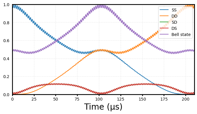
Correlated Phase#
Construct the system#
# Construct the system
ca = Ca40([("S1/2", -1/2, "S"), ("D5/2", -1/2, "D")])
laser1 = Laser(pointing=[(1, 1.), (2, 1.)])
laser2 = Laser(pointing=[(1, 1.), (2, 1.)])
chain = LinearChain(
        ions=[ca, ca], comfrequencies=(x=3e6,y=3e6,z=2.5e5), selectedmodes=(;z=[1])
    )
chamber = Chamber(iontrap=chain, B=6e-4, Bhat=(x̂ + ẑ)/√2, lasers=[laser1, laser2]);
Set the laser parameters#
mode = zmodes(chamber)[1]
ν = frequency(mode)

ϵ = 10e3
d = 350 # corrects for AC stark shift from single-photon coupling to sidebands

wavelength_from_transition!(laser1, ca, ("S", "D"), chamber)
detuning!(laser1, ν + ϵ - d)
polarization!(laser1, x̂)
wavevector!(laser1, ẑ)

wavelength_from_transition!(laser2, ca, ("S", "D"), chamber)
detuning!(laser2, -ν - ϵ + d)
polarization!(laser2, x̂)
wavevector!(laser2, ẑ)

η = abs(lambdicke(mode, ca, laser1))
pi_time = η / ϵ  # setting 'resonance' condition: ηΩ = 1/2ϵ
intensity_from_pitime!(1, pi_time, 1, ("S", "D"), chamber)
intensity_from_pitime!(2, pi_time, 1, ("S", "D"), chamber);
Build the Hamiltonian / solve the system#
# setup the Hamiltonian
h = hamiltonian(chamber, timescale=1e-6, lamb_dicke_order=1, rwa_cutoff=Inf);
# solve system
@time tout, sol = timeevolution.schroedinger_dynamic(0:0.1:210, ca["S"] ⊗ ca["S"] ⊗ mode[0], h);
0.473047 seconds (2.94 M allocations: 104.585 MiB, 8.98% gc time)
Plot results#
SS = ionprojector(chamber, "S", "S")
DD = ionprojector(chamber, "D", "D")
SD = ionprojector(chamber, "S", "D")
DS = ionprojector(chamber, "D", "S")
bell_state = dm((ca["S"] ⊗ ca["S"] + 1im * ca["D"] ⊗ ca["D"])/√2) ⊗ one(mode)

# compute expectation values
prob_SS = expect(SS, sol)  # 𝔼(|S⟩|S⟩)
prob_DD = expect(DD, sol)  # 𝔼(|D⟩|D⟩)
prob_SD = expect(SD, sol)  # 𝔼(|S⟩|D⟩)
prob_DS = expect(DS, sol)  # 𝔼(|D⟩|S⟩)
prob_bell = expect(bell_state, sol)  # 𝔼((|S⟩|S⟩ + i|D⟩|D⟩)/√2)

# plot results
plt.plot(tout, prob_SS, label="SS")
plt.plot(tout, prob_DD, label="DD")
plt.plot(tout, prob_SD, label="SD")
plt.plot(tout, prob_DS, label="DS")
plt.plot(tout, prob_bell, label="Bell state")
plt.xlim(tout[1], tout[end])
plt.ylim(0, 1)
plt.legend(loc=1)
plt.xlabel("Time (μs)");
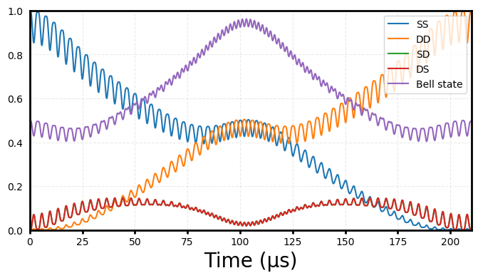
Anti-correlated phase#
Update phase#
phase!(laser1, -π/2)
phase!(laser2, π/2);
Build the Hamiltonian / solve the system#
h = hamiltonian(chamber, timescale=1e-6, lamb_dicke_order=1, rwa_cutoff=Inf);
@time tout, sol = timeevolution.schroedinger_dynamic(0:0.1:210, ca["S"] ⊗ ca["S"] ⊗ mode[0], h);
0.396818 seconds (3.24 M allocations: 115.232 MiB, 9.90% gc time)
Plot results#
# compute expectation values
prob_SS = expect(SS, sol)  # 𝔼(|S⟩|S⟩)
prob_DD = expect(DD, sol)  # 𝔼(|D⟩|D⟩)
prob_SD = expect(SD, sol)  # 𝔼(|S⟩|D⟩)
prob_DS = expect(DS, sol)  # 𝔼(|D⟩|S⟩)
prob_bell = expect(bell_state, sol)  # 𝔼((|S⟩|S⟩ + i|D⟩|D⟩)/√2)

# plot results
plt.plot(tout, prob_SS, label="SS")
plt.plot(tout, prob_DD, label="DD")
plt.plot(tout, prob_SD, label="SD")
plt.plot(tout, prob_DS, label="DS")
plt.plot(tout, prob_bell, label="Bell state")
plt.xlim(tout[1], tout[end])
plt.ylim(0, 1)
plt.legend(loc=1)
plt.xlabel("Time (μs)");
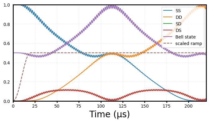
Anti-correlated phase with ramped laser intensity#
Update intensity profile#
I = intensity_from_pitime(1, pi_time, 1, ("S", "D"), chamber)
# Simple amplitude ramping function
Ω = t -> t < 20 ? sin(2π * t / 80)^2 : 1

intensity!(laser1, t -> I*Ω(t)^2)
intensity!(laser2, t -> I*Ω(t)^2);
Build the Hamiltonian / solve the system#
h = hamiltonian(chamber, timescale=1e-6, lamb_dicke_order=1, rwa_cutoff=Inf);
@time tout, sol = timeevolution.schroedinger_dynamic(0:0.1:220, ca["S"] ⊗ ca["S"] ⊗ mode[0], h);
0.794465 seconds (5.62 M allocations: 159.405 MiB, 10.27% gc time, 4.17% compilation time)
Plot results#
# compute expectation values
prob_SS = expect(SS, sol)  # 𝔼(|S⟩|S⟩)
prob_DD = expect(DD, sol)  # 𝔼(|D⟩|D⟩)
prob_SD = expect(SD, sol)  # 𝔼(|S⟩|D⟩)
prob_DS = expect(DS, sol)  # 𝔼(|D⟩|S⟩)
prob_bell = expect(bell_state, sol)  # 𝔼((|S⟩|S⟩ + i|D⟩|D⟩)/√2)

# plot results
plt.plot(tout, prob_SS, label="SS")
plt.plot(tout, prob_DD, label="DD")
plt.plot(tout, prob_SD, label="SD")
plt.plot(tout, prob_DS, label="DS")
plt.plot(tout, prob_bell, label="Bell state")
plt.plot(
        tout, @.(Ω(tout) / 2),
        linestyle="--", label="scaled ramp"
    )
plt.xlim(tout[1], tout[end])
plt.ylim(0, 1)
plt.legend(loc=1)
plt.xlabel("Time (μs)");
Bibliography#
- Roo08
Christian F Roos. Ion trap quantum gates with amplitude-modulated laser beams. New Journal of Physics, 10(1):013002, jan 2008. URL: https://doi.org/10.1088%2F1367-2630%2F10%2F1%2F013002, doi:10.1088/1367-2630/10/1/013002.